Creating and editing curves

The purpose of this tutorial is to demonstrate how to inner and outer boundary curve chains. By a "chain" we mean a closed curve that is composed of multiple pieces. Each chain can be a combination of different curve types, e.g., a circular arc can connect to a spline. It also shows how to modify, remove, and add new pieces to an existing curve chain. The undo and redo capabilities of the interactive mesh tool are briefly discussed. The outer and inner boundary curves, background grid as well as the mesh will be visualized for quality inspection.

Synopsis

This tutorial demonstrates how to:

• Create and edit an outer boundary chain.
• Create and edit an inner boundary chain.
• Add the background grid when an outer boundary curve is present.
• Visualize an interactive mesh project.
• Discuss undo / redo capabilities.
• Construct and add parametric spline curves.
• Construct and add a curve from parametric equations.
• Construct and add straight line segments.
• Construct and add circular arc segments.

Initialization

From a Julia REPL we load the HOHQMesh package as well as GLMakie, a backend of Makie.jl, to visualize the curves, mesh, etc. from the interactive tool.

julia> using GLMakie, HOHQMesh

Now we are ready to interactively generate unstructured quadrilateral meshes!

We create a new project with the name "sandbox" and assign "out" to be the folder where any output files from the mesh generation process will be saved. By default, the output files created by HOHQMesh will carry the same name as the project. For example, the resulting HOHQMesh control file from this tutorial will be named sandbox.control. If the folder out does not exist, it will be created automatically in the current file path.

sandbox_project = newProject("sandbox", "out")

Add the outer boundary chain

We first create the outer boundary curve chain that is composed of three pieces

1. Straight line segment from $(0, -7)$ to $(5, 3)$.
2. Half-circle arc of radius $r=5$ centered at $(0, 3)$.
3. Straight line segment from $(-5, 3)$ to $(0, -7)$.

Each segment of the curve is created separately. The straight line segments are made with the function newEndPointsLineCurve and given unique names:

outer_line1 = newEndPointsLineCurve("Line1",          # curve name
                                    [0.0, -7.0, 0.0], # start point
                                    [5.0,  3.0, 0.0]) # end point

outer_line2 = newEndPointsLineCurve("Line2",          # curve name
                                    [-5.0, 3.0, 0.0], # start point
                                    [0.0, -7.0, 0.0]) # end point

To create the circle arc we use the function newCircularArcCurve where we specify a name for the curve as well as the radius and center of the circle. The arc can have an arbitrary length dictated by the start and end angle, e.g., for a half-circle we take the angle to vary from $0$ to $180$ degrees.

outer_arc = newCircularArcCurve("Arc",           # curve name
                                [0.0, 3.0, 0.0], # center
                                5.0,             # radius
                                0.0,             # start angle
                                180.0,           # end angle
                                "degrees")       # units for angle

We use "degrees" to set the angle bounds, but "radians" can also be used. The name of the curve stored in the dictionary outer_arc is assigned to be "Arc".

The curve names "Line1", "Line2", and "Arc" are the labels that HOHQMesh will give to these boundary curve segments in the resulting mesh file.

The three curve segments stored in the variables outer_line1, outer_line2, and outer_arc are then added to the sandbox_project with a counter-clockwise orientation as required by HOHQMesh.

addCurveToOuterBoundary!(sandbox_project, outer_line1)
addCurveToOuterBoundary!(sandbox_project, outer_arc)
addCurveToOuterBoundary!(sandbox_project, outer_line2)

Add a background grid

HOHQMesh requires a background grid for the mesh generation process. This background grid sets the base resolution of the desired mesh. HOHQMesh will automatically subdivide from this background grid near sharp features of any curved boundaries.

For a domain bounded by an outer boundary curve, this background grid is set by indicating the desired element size in the $x$ and $y$ directions. To start, we set the background grid for sandbox_project to have elements with side length one in each direction

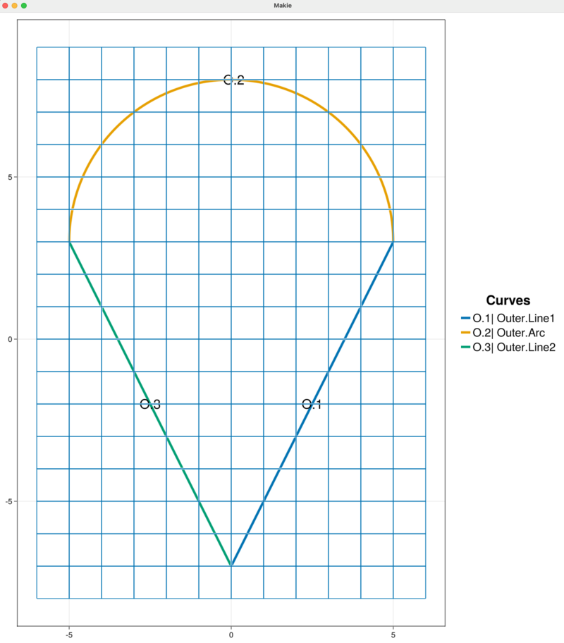
addBackgroundGrid!(sandbox_project, [1.0, 1.0, 0.0])

We visualize the outer boundary curve chain and background grid with the following

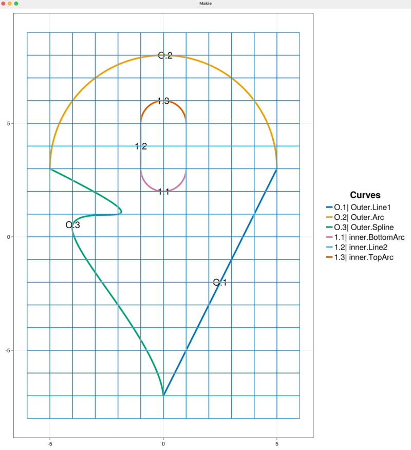
plotProject!(sandbox_project, MODEL+GRID)

Here, we take the sum of the keywords MODEL and GRID in order to simultaneously visualize the outer boundary and background grid. The resulting plot is given below. The chain of outer boundary curves is called "Outer" and it contains three curve segments "Line1", "Arc", and "Line2" labeled in the figure by O.1, O.2, and O.3, respectively.

Edit the outer boundary chain

Suppose that the domain boundary requires a curved segment instead of the straight line "Line2". We will replace this line segment in the outer boundary chain with a cubic spline.

First, we remove the "Line2" curve from the "Outer" chain with the command

removeOuterBoundaryCurveWithName!(sandbox_project, "Line2")

removeOuterBoundaryCurveAtIndex!(sandbox_project, 3)

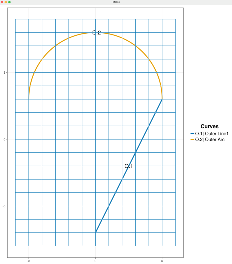
The plot automatically updates and we see that the outer boundary is open and contains two segments: "Line1" and "Arc".

Next, we create a parametric cubic spline curve from a given set of data points. In order to make a closed outer boundary chain the cubic spline must begin at the endpoint of the curve "Arc" and end at the first point of the curve "Line1". This ensures that the new spline curve connects into the boundary curve chain with the correct orientation. To create a parametric spline curve we directly provide data points in the code. These points take the form [t, x, y, z] where t is the parameter variable that varies between $0$ and $1$. The spline curve constructor newSplineCurve also takes the number of points as an input argument.

spline_data = [ [0.0  -5.0  3.0 0.0]
                [0.25 -2.0  1.0 0.0]
                [0.5  -4.0  0.5 0.0]
                [0.75 -2.0 -3.0 0.0]
                [1.0   0.0 -7.0 0.0] ]
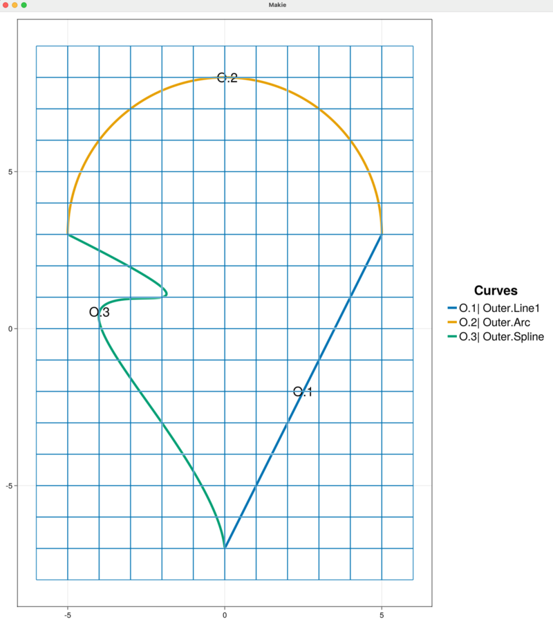
outer_spline = newSplineCurve("Spline", 5, spline_data)

Now we add the spline curve outer_spline into the sandbox_project.

addCurveToOuterBoundary!(sandbox_project, outer_spline)

The figure updates automatically to display the "Outer" boundary chain with the new "Spline" curve labeled O.3.

Add an inner boundary chain

We create a pill shaped inner boundary curve chain composed of four pieces

1. Straight line segment from $(1, 5)$ to $(1, 3)$.
2. Half-circle arc of radius $r=1$ centered at $(0, 3)$.
3. Straight line segment from $(-1, 3)$ to $(-1, 5)$.
4. Half-circle arc of radius $r=1$ centered at $(0, 5)$.

Similar to the construction of the "Outer" boundary chain, each segment of this inner boundary chain is created separately. The straight line segments are made with the function newEndPointsLineCurve and given unique names:

inner_line1 = newEndPointsLineCurve("Line1",         # curve name
                                    [1.0, 5.0, 0.0], # start point
                                    [1.0, 3.0, 0.0]) # end point

inner_line2 = newEndPointsLineCurve("Line2",          # curve name
                                    [-1.0, 3.0, 0.0], # start point
                                    [-1.0, 5.0, 0.0]) # end point

To create the circle arcs we use the function newCircularArcCurve where we specify a name for the curve as well as the radius and center of the circle. In order to create an inner curve chain with counter-clockwise orientation the angle for the bottom half-circle arc centered at $(0, 3)$ varies from $0$ to $-180$ degrees. The top half-circle arc centered at $(0, 5)$ has an angle that varies from $180$ to $0$ degrees. The construction of the two circle arcs are

inner_bottom_arc = newCircularArcCurve("BottomArc",     # curve name
                                       [0.0, 3.0, 0.0], # center
                                       1.0,             # radius
                                       0.0,             # start angle
                                       -pi,             # end angle
                                       "radians")       # units for angle

inner_top_arc = newCircularArcCurve("TopArc",        # curve name
                                    [0.0, 5.0, 0.0], # center
                                    1.0,             # radius
                                    180.0,           # start angle
                                    0.0,             # end angle
                                    "degrees")       # units for angle

Note, we use "radians" to set the angle bounds for inner_bottom_arc and "degrees" for the angle bounds of inner_top_arc.

The curve names "Line1", "Line2", "BottomArc", and "TopArc" are the labels that HOHQMesh will give to these inner boundary curve segments in the resulting mesh file.

The four curve segments stored in the variables inner_line1, inner_line2, inner_bottom_arc and outer_arc are added to the sandbox_project in counter-clockwise order as required by HOHQMesh.

addCurveToInnerBoundary!(sandbox_project, inner_line1,      "inner")
addCurveToInnerBoundary!(sandbox_project, inner_bottom_arc, "inner")
addCurveToInnerBoundary!(sandbox_project, inner_line2,      "inner")
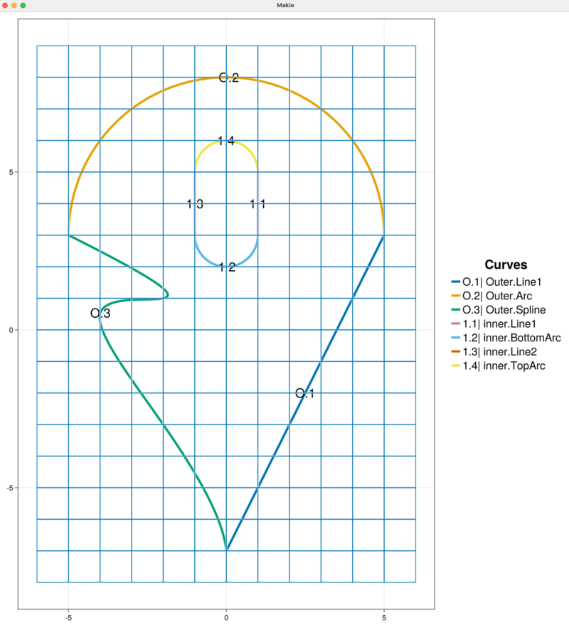
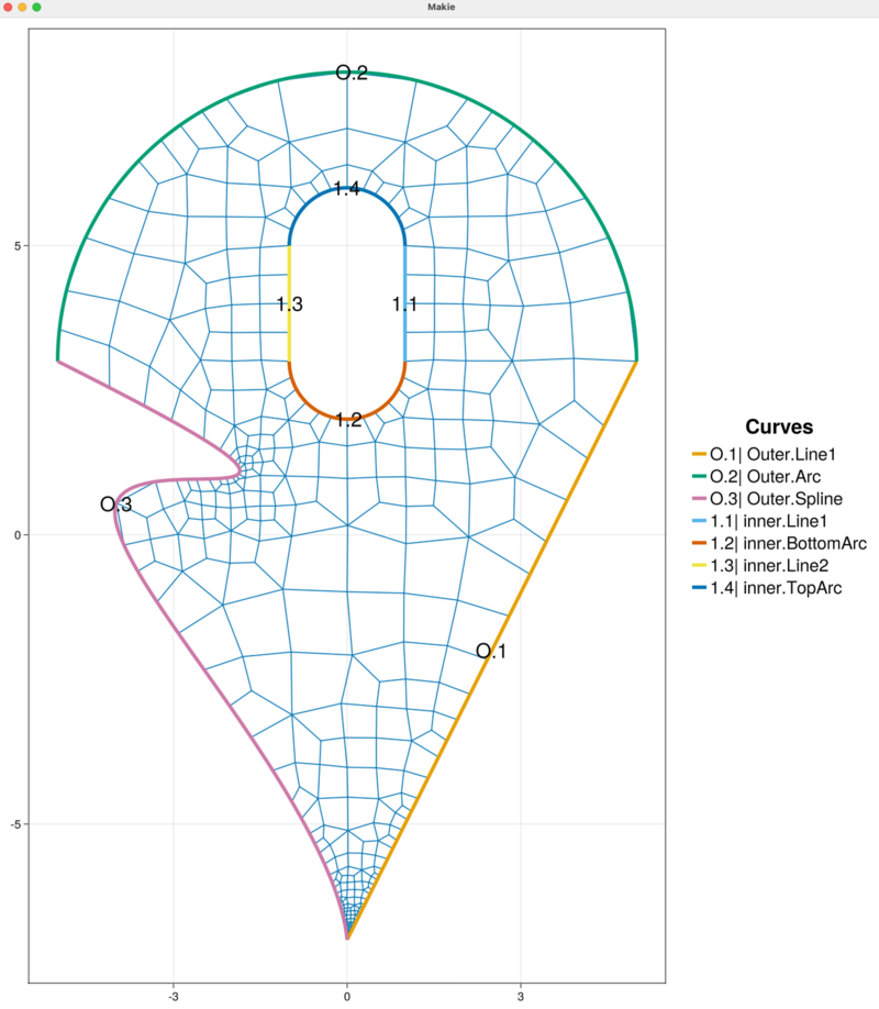
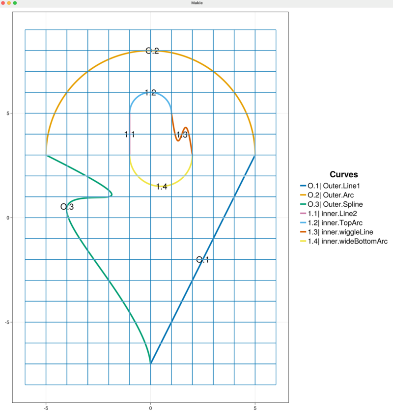
addCurveToInnerBoundary!(sandbox_project, inner_top_arc,    "inner")

This inner boundary chain name "inner" is used internally by HOHQMesh. The visualization of the background grid automatically detects that curves have been added to the sandbox_project and the plot is updated, as shown below. The chain for the inner boundary curve chain is called inner and it contains a four curve segments "Line1", "BottomArc", "Line2", and "TopArc" labeled in the figure by 1.1, 1.2, 1.3, and 1.4, respectively.

Generate the mesh

We next generate the mesh from the information contained in the sandbox_project. This will output the following files to the out folder:

• sandbox.control: A HOHQMesh control file for the current project.
• sandbox.tec: A TecPlot formatted file to visualize the mesh with other software, e.g., ParaView.
• sandbox.mesh: A mesh file with format ISM-V2 (the default format).

To do this we execute the command

generate_mesh(sandbox_project)

 *******************
 2D Mesh Statistics:
 *******************
    Total time             =    7.5414000000000009E-002
    Number of nodes        =          511
    Number of Edges        =          933
    Number of Elements     =          422
    Number of Subdivisions =            7

 Mesh Quality:
         Measure         Minimum         Maximum         Average  Acceptable Low Acceptable High       Reference
     Signed Area      0.00002932      1.17335568      0.18813138      0.00000000    999.99900000      1.00000000
    Aspect Ratio      1.00953438      2.30790024      1.31439620      1.00000000    999.99900000      1.00000000
       Condition      1.00041663      2.41773865      1.21024584      1.00000000      4.00000000      1.00000000
      Edge Ratio      1.01673809      3.68828437      1.59413340      1.00000000      4.00000000      1.00000000
        Jacobian      0.00001750      1.13820387      0.14143901      0.00000000    999.99900000      1.00000000
   Minimum Angle     32.22733574     89.35690571     68.75321248     40.00000000     90.00000000     90.00000000
   Maximum Angle     90.61089476    152.37947944    113.36221513     90.00000000    135.00000000     90.00000000
       Area Sign      1.00000000      1.00000000      1.00000000      1.00000000      1.00000000      1.00000000

The call to generate_mesh also prints mesh quality statistics to the screen and updates the visualization. The background grid is removed from the visualization when the mesh is generated.

Delete the existing mesh

In preparation of edits we will make to the inner boundary chain we remove the current mesh from the plot and re-plot the model curves and background grid. Note, this step is not required, but it helps avoid confusion when editing several curves.

remove_mesh!(sandbox_project)
updatePlot!(sandbox_project, MODEL+GRID)

The remove_mesh! command deletes the mesh information from the sandbox_project as well as the mesh file sandbox.mesh, control file sandbox.control, plot file sandbox.tec, and mesh statistics file sandbox.txt from the out folder.

Edit an inner boundary chain

Suppose that the inner boundary actually requires a curved segment instead of the straight line "Line1". We will replace this line segment in the inner boundary chain with an oscillating segment construct from a set of parametric equations. In doing so, it will also be necessary to remove the BottomArc and replace it with a new, wider circular arc segment.

We remove the "Line1" curve from the inner chain with the command

removeInnerBoundaryCurve!(sandbox_project, "Line1", "inner")

removeInnerBoundaryCurveAtIndex!(sandbox_project, 1, "inner")

With either removal strategy, the plot automatically updates. We see that the inner boundary is open and contains three segments: "BottomArc", "Line2", and "TopArc". Note that the index of the remaining curves has changed as shown below.

undoActionName()
"Remove Inner Boundary Curve"

undo()
"Undo Remove Inner Boundary Curve"

The new inner curve segment will be an oscillating line given by the parametric equations

\[ \begin{aligned} x(t) &= t + 1,\\[0.2cm] y(t) &= -2t + 5 - \frac{3}{2} \cos(\pi t) \sin(\pi t),\\[0.2cm] z(t) &= 0 \end{aligned} \qquad t\in[0,1]\]

Parametric equations in HOHQMesh can be any legitimate equation and use intrinsic functions available in Fortran, e.g., $\sin$, $\cos$, exp. The constant pi is available for use. The following commands create a new curve for the parametric equations above

xEqn = "x(t) = t + 1"
yEqn = "y(t) = -2 * t + 5 - 1.5 * cos(pi * t) * sin(pi * t)"
zEqn = "z(t) = 0.0"
inner_eqn = newParametricEquationCurve("wiggleLine", xEqn, yEqn, zEqn)

The name of this new curve is assigned to be "wiggleLine". We add this new curve to the "inner" chain.

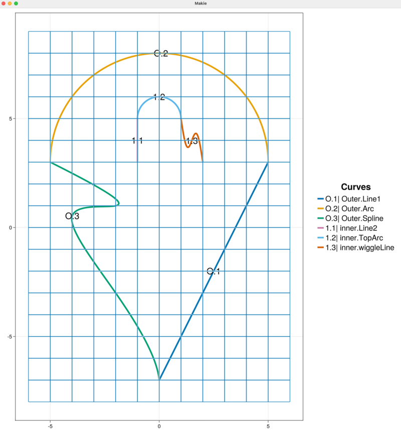
addCurveToInnerBoundary!(sandbox_project, inner_eqn, "inner")

The automatically updated figure now shows:

We see from the figure that this parametric equation curve starts at the point $(1,5)$ and, therefore, matches the end point of the existing curve "TopArc" present in the "inner" chain. However, the parametric equation curve ends at the point $(2,3)$ which does not match the "BottomArc" curve. So, the inner boundary chain remains open.

To create a closed boundary curve we must remove the "BottomArc" curve and replace it with a wider half-circle arc segment. This new half-circle arc must start at the point $(2, 3)$ and end at the point $(-1, 3)$ to close the inner chain and guarantee the chain is oriented counter-clockwise. So, we first remove the "BottomArc" from the "inner" chain.

removeInnerBoundaryCurve!(sandbox_project, "BottomArc", "inner")

The figure updates to display the "inner" curve chain with three segments. Note that the inner curve chain indexing has, again, been automatically adjusted.

A half-circle arc that joins the points $(2, 3)$ and $(-1, 3)$ has a radius $r=1.5$, is centered at $(0.5, 3)$ and has an angle that vaires from $0$ to $-180$. We construct this circle arc and directly add it to the sandbox_project.

new_bottom_arc = newCircularArcCurve("wideBottomArc", # curve name
                                     [0.5, 3.0, 0.0], # center
                                     1.5,             # radius
                                     0.0,             # start angle
                                     -pi,             # end angle
                                     "radians")       # units for angle
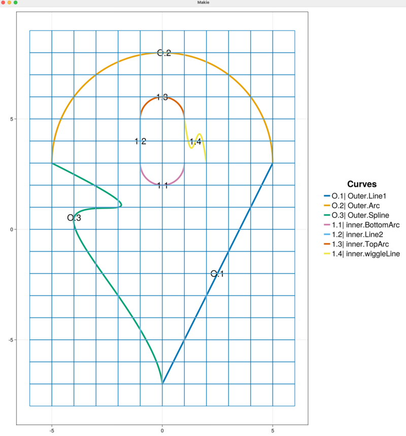
addCurveToInnerBoundary!(sandbox_project, new_bottom_arc, "inner")

The updated plot now gives the modified, closed inner curve chain that now contains four curve segments "Line2", "TopArc", "wiggleLine", and "wideBottomArc" labeled in the figure by 1.1, 1.2, 1.3, and 1.4, respectively.

Regenerate the mesh

With the modifications to the inner curve chain complete we can regenerate the mesh. This will create a new sandbox.mesh file and overwrite the existing sandbox.control and sandbox.tec files in the out directory.

generate_mesh(sandbox_project)

 *******************
 2D Mesh Statistics:
 *******************
    Total time             =   0.11353599999999998
    Number of nodes        =          712
    Number of Edges        =         1308
    Number of Elements     =          596
    Number of Subdivisions =            7

 Mesh Quality:
         Measure         Minimum         Maximum         Average  Acceptable Low Acceptable High       Reference
     Signed Area      0.00002932      1.15661960      0.12823902      0.00000000    999.99900000      1.00000000
    Aspect Ratio      1.01050856      3.14732001      1.34260027      1.00000000    999.99900000      1.00000000
       Condition      1.00037771      2.59434067      1.22850175      1.00000000      4.00000000      1.00000000
      Edge Ratio      1.02744717      3.68828437      1.64751502      1.00000000      4.00000000      1.00000000
        Jacobian      0.00001750      1.13149451      0.09443920      0.00000000    999.99900000      1.00000000
   Minimum Angle     31.87236189     89.33988565     67.86178629     40.00000000     90.00000000     90.00000000
   Maximum Angle     90.44177106    157.27121105    114.35699650     90.00000000    135.00000000     90.00000000
       Area Sign      1.00000000      1.00000000      1.00000000      1.00000000      1.00000000      1.00000000

The visualization updates automatically and the background grid is removed after when the mesh is generated.

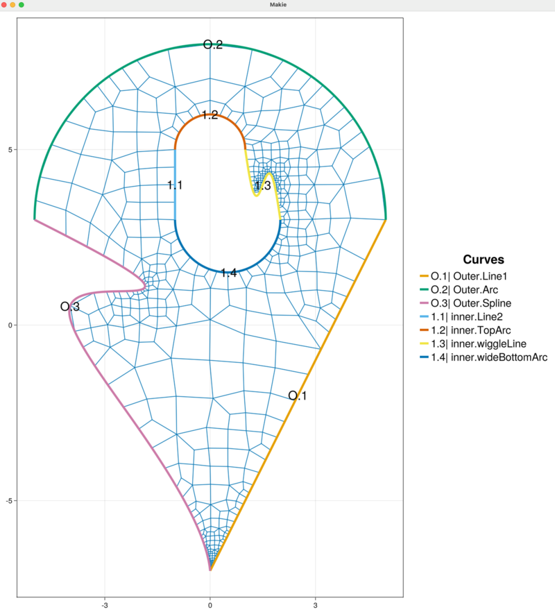
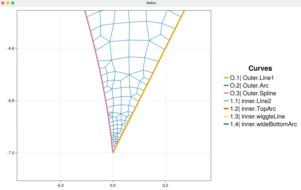
Inspecting the mesh we see that the automatic subdivision in HOHQMesh does well to capture the sharp corners and fine features of the curved inner and outer boundaries. For example, we zoom into sharp corner at the bottom of the domain and see that, although small, the elements in this region maintain a good quadrilateral shape.

Summary

In this tutorial we demonstrated how to:

• Create and edit an outer boundary chain.
• Create and edit an inner boundary chain.
• Add the background grid when an outer boundary curve is present.
• Visualize an interactive mesh project.
• Discuss undo / redo capabilities.
• Construct and add parametric spline curves.
• Construct and add a curve from parametric equations.
• Construct and add straight line segments.
• Construct and add circular arc segments.

For completeness, we include a script with all the commands to generate the mesh displayed in the final image. Note, we do not include the plotting in this script.

# Interactive mesh with modified outer and inner curve chains
#
# Create inner / outer boundary chains composed of the four
# available HOHQMesh curve types.
#
# Keywords: outer boundary, inner boundary, parametric equations,
#           circle arcs, cubic spline, curve removal
using HOHQMesh

# Instantiate the project
sandbox_project = newProject("sandbox", "out")

# Add the background grid
addBackgroundGrid!(sandbox_project, [1.0, 1.0, 0.0])

# Create and add the original outer boundary curves
outer_line1 = newEndPointsLineCurve("Line1", [0.0, -7.0, 0.0], [5.0,  3.0, 0.0])
outer_line2 = newEndPointsLineCurve("Line2", [-5.0, 3.0, 0.0], [0.0, -7.0, 0.0])
outer_arc = newCircularArcCurve("Arc",  [0.0, 3.0, 0.0], 5.0, 0.0, 180.0, "degrees")

addCurveToOuterBoundary!(sandbox_project, outer_line1)
addCurveToOuterBoundary!(sandbox_project, outer_arc)
addCurveToOuterBoundary!(sandbox_project, outer_line2)

# Modify the outer boundary to have a spline instead of a straight line
removeOuterBoundaryCurveWithName!(sandbox_project, "Line2")

spline_data = [ [0.0  -5.0  3.0 0.0]
                [0.25 -2.0  1.0 0.0]
                [0.5  -4.0  0.5 0.0]
                [0.75 -2.0 -3.0 0.0]
                [1.0   0.0 -7.0 0.0] ]
outer_spline = newSplineCurve("Spline", 5, spline_data)
addCurveToOuterBoundary!(sandbox_project, outer_spline)

# Create and add the inner boundary curves
inner_line1 = newEndPointsLineCurve("Line1", [1.0, 5.0, 0.0], [1.0, 3.0, 0.0])
inner_line2 = newEndPointsLineCurve("Line2", [-1.0, 3.0, 0.0], [-1.0, 5.0, 0.0])
inner_bottom_arc = newCircularArcCurve("BottomArc", [0.0, 3.0, 0.0], 1.0, 0.0, -pi, "radians")
inner_top_arc = newCircularArcCurve("TopArc", [0.0, 5.0, 0.0], 1.0, 180.0, 0.0, "degrees")

addCurveToInnerBoundary!(sandbox_project, inner_line1, "inner")
addCurveToInnerBoundary!(sandbox_project, inner_bottom_arc, "inner")
addCurveToInnerBoundary!(sandbox_project, inner_line2, "inner")
addCurveToInnerBoundary!(sandbox_project, inner_top_arc, "inner")

# Generate a mesh
generate_mesh(sandbox_project)

# Delete the existing mesh before modifying the inner boundary curve chain
remove_mesh!(sandbox_project)

# Modify the inner boundary curve with an oscillatory line and a new circle arc
removeInnerBoundaryCurve!(sandbox_project, "Line1", "inner")
removeInnerBoundaryCurve!(sandbox_project, "BottomArc", "inner")

xEqn = "x(t) = t + 1"
yEqn = "y(t) = -2 * t + 5 - 1.5 * cos(pi * t) * sin(pi * t)"
zEqn = "z(t) = 0.0"
inner_eqn = newParametricEquationCurve("wiggleLine", xEqn, yEqn, zEqn)

new_bottom_arc = newCircularArcCurve("wideBottomArc", [0.5, 3.0, 0.0], 1.5, 0.0, -pi, "radians")

addCurveToInnerBoundary!(sandbox_project, inner_eqn, "inner")
addCurveToInnerBoundary!(sandbox_project, new_bottom_arc, "inner")

# Regenerate the final mesh
generate_mesh(sandbox_project)